Blog
How to Compare Two Excel Sheets: =, Conditional Formatting, VLOOKUP, and MATCH
 Mike Yi · Jul 22, 2026
Comparing two sheets is one of those tasks that sounds trivial until the row count climbs past a hundred. Scanning line by line to catch every mismatch is slow, and it is exactly the kind of repetitive work where your eyes start skipping things, especially values that look almost identical.
This guide walks through four ways to compare two Excel sheets: the = operator for a quick TRUE/FALSE check, conditional formatting to highlight differences visually, and VLOOKUP or MATCH to find values that exist in one sheet but not the other.
Why Comparing Sheets by Eye Falls Apart
Comparing two months of revenue, or two headcount lists from different departments, are the kinds of tasks that come up constantly. The problem is that manual comparison stops being reliable the moment a sheet has more than a hundred or so rows.
Scrolling back and forth between two sheets makes it easy to lose your place, and once the rows drift out of alignment, you end up comparing completely unrelated values without realizing it. The larger the dataset, the more this fatigue compounds, and the more small discrepancies slip through. Fixing that requires a formula-based approach instead of your eyes.
Compare Two Columns with the = Operator
The simplest way to compare two Excel columns is the = operator: no function required, just an instant TRUE or FALSE for every row.
Basic Syntax
If the values you want to compare sit in column B and column C, enter this formula in column D:
=B2=C2
The result is TRUE if the values match and FALSE if they do not. Drag the formula down and you get a full column of comparisons in seconds.

In the example, apples and pears show TRUE because their January and February prices did not change ($10 and $20). Avocados, limes, oranges, lemons, and grapes all show FALSE, meaning their price moved between the two months.
Filtering to the Rows That Actually Changed
A column full of TRUE and FALSE is not very useful until you filter it. Apply a filter to the result column and keep only FALSE, and you are left with just the rows where something changed.
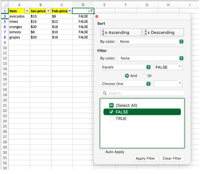
Filtering down to FALSE turns a wall of TRUE/FALSE values into a short, actionable list, in this case five items whose price changed month over month.
The Case-Sensitivity Trap
The = operator is not case-sensitive: "Apple" and "apple" both evaluate to TRUE. If you need an exact, case-sensitive comparison, use EXACT instead:
=EXACT(A2,B2)
Also watch for numbers stored as text. A value that looks numeric but is stored as text will often return FALSE against a real number, so it is worth normalizing data types before you compare.
Highlight Differences with Conditional Formatting
The = operator gives you an accurate answer, but a column of TRUE/FALSE is not exactly easy to scan. Conditional formatting solves that by coloring the cells that differ, so mismatches jump out visually instead of requiring you to read every row.
Setting It Up Step by Step
Step 1: Select the range to compare
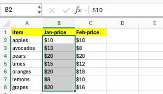
Select the column or range you want to check for differences. Here, that is B2:B8.
Step 2: Open the Conditional Formatting menu

Go to Home > Conditional Formatting > New Rule.
Step 3: Enter the formula
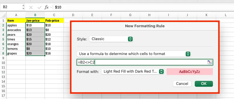
Choose Use a formula to determine which cells to format, then enter:
=B2<>C2
Set a fill or font color, and every cell where the value differs from its neighbor gets highlighted automatically.
Highlighting Differences Across Two Separate Sheets

If what you are comparing lives on a different sheet, include the sheet name in the formula:
=B2<>Sheet2!B2
This highlights any cell in Sheet1's column B whose value does not match the corresponding cell in Sheet2's column B.

Apples and pears stay unhighlighted because their values matched. The five rows that changed are colored automatically, and the highlight updates itself the moment either sheet's data changes.
The Limits of Conditional Formatting
Conditional formatting is great for a visual scan, but it does not let you extract or list the differences separately. If you have a lot of highlighted cells, or you need a clean list of what changed, pair it with VLOOKUP or MATCH.
Find Missing Values with VLOOKUP
VLOOKUP is the function most people reach for when comparing two sheets, and it is especially good at catching missing or dropped records: values that exist on one side but not the other.
The Comparison Formula Structure
The base syntax is:
=VLOOKUP(lookup_value, lookup_range, column_number, 0)
For comparison purposes, the last argument must always be 0 (exact match).
Finding a Value That Disappeared
Say you have an employee roster for 2025 and 2026, and you want to know whether each employee's department changed, or whether they disappeared from the list entirely.
=VLOOKUP(A6,'2026'!$A$2:$C$11,3,0)

If the value exists, VLOOKUP returns it directly. If it does not, you get a #N/A error. In the example, every employee's 2025 and 2026 department match except Lisa, whose ID does not appear anywhere in the 2026 sheet, so the formula returns #N/A.
Wrapping the formula in IFERROR lets you replace that #N/A with a label that actually means something, like flagging Lisa as no longer active:
=IFERROR(VLOOKUP(A6,'2026'!$A$2:$C$11,3,0),"Resigned")

Why VLOOKUP Comparisons Return #N/A
If you are seeing more #N/A results than expected, check these three things first:
- Mismatched data types: one side stored as a number, the other as text
- Hidden whitespace: invisible spaces before or after the value
- Wrong range: the lookup range does not actually cover the value you are searching for
Wrapping your lookup value in TRIM before comparing clears up a large share of these errors.
Compare Sheets with MATCH
MATCH returns the position of a value within a range rather than a value itself. Since it does not require a column number, it tends to be more flexible for comparison work than VLOOKUP.
Basic Structure
=MATCH(lookup_value, lookup_range, 0)
If the value exists, MATCH returns its position as a number. If it does not, you get #N/A, exactly like VLOOKUP.

Here, MATCH confirms the same finding as VLOOKUP: every employee from the 2025 list is found in the 2026 list except Lisa, who returns #N/A because her ID is no longer present.
VLOOKUP vs MATCH: Which One to Use
| Situation | Recommended function |
|---|---|
| Checking whether a specific value exists in another sheet | VLOOKUP |
| Just confirming existence, quickly | MATCH |
| Comparing multiple columns at once | INDEX + MATCH |
| Data where column positions shift often | MATCH |
Comparing Large Datasets
Once a dataset grows, the order you work in matters more than which function you pick.
Getting Your Comparison Order Right
Step 1: Standardize the sort order. Sort both sheets ascending by the same key column, such as an ID or code. If the sort order differs between sheets, matching values end up in different positions and comparison breaks down.
Step 2: Standardize the data type. Make sure numbers and text are not mixed. TRIM and CLEAN remove stray whitespace and hidden characters.
Step 3: Compare the key column first. Rather than comparing everything at once, check the identifying column (like an ID) first to catch missing or added rows before you go any further.
Pulling Out Just the Differences
Filtering the = operator or VLOOKUP result down to FALSE or a missing-value label isolates only the rows that changed. Paste that filtered set into a new sheet, and you have a clean list of differences with nothing else in the way.
Making Repeat Comparisons Faster
If you are comparing the same kind of data structure every month, save a sheet with the comparison formulas already in place as a template. Paste in the new data and the formulas recalculate automatically, so you are never starting from scratch.
A Faster Way to Compare Sheets with inline AI

Knowing these four methods is one thing. Typing the right formula, setting up conditional formatting, and cleaning up the result column every time your data structure shifts slightly is the part that eats your afternoon.
inline AI reads your table structure automatically and finds the differences between two sheets for you, building the conditional formatting rule or comparison formula without you typing a single one. Ask in plain English, and it handles the ranges, the sheet references, and the formatting.
It runs locally on your PC, so your data stays on your machine with nothing uploaded to the cloud.
If comparing sheets is a recurring part of your month, let inline AI handle the repetitive setup so you can spend that time on the analysis instead.
Download your AI Coworker for Excel